Multiple time meshes for MILP energy systems modelling
This is a direct continuation of the post on heterogeneous time meshes, which exploited the fact that temporal resolution is not equally valuable at every time of the year. In this post, we exploit the fact that temporal resolution is not equally valuable in every part of the system.
Let’s first define a node as an abstract, passive place where the balance of flows is enforced. A node can represent many things including a bidding zone in a regional power system, a hydrogen pipe in a hydrogen system, or a wire in an electric device. One node is only associated with one carrier. The active counterpart of the node is the component, which generates and/or consumes flows. There are many systems that require modelling of multiple nodes. In one system, multiple nodes can represent multiple geographic or market zones, multiple parts of a system supporting different carriers, etc.
A convention that I like, and that is applied in Nosy, is that components are connected only to nodes, and vice versa.
Let’s model an electricity and hydrogen system composed of PV, battery, electricity consumption, electrolyser, long-term hydrogen storage, and hydrogen consumption. The capacity of every component is an investment decision, except for consumption. Let’s also assume, for simplicity, that the electricity and hydrogen consumption profiles are flat. The full example is available in Nosy’s documentation.

The levels of the battery and hydrogen storage during the first week of June are shown below, both evaluated using hourly time meshes. The data is synthetic, so the shape of the curves is more regular than with real-world data, but it still captures the essence of the dynamics.
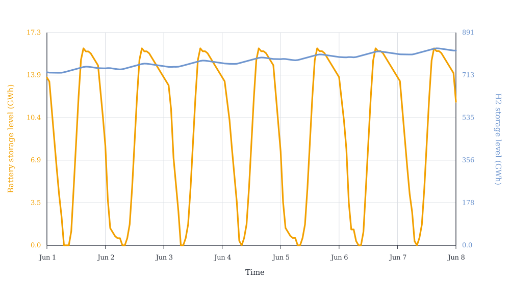
Let’s analyze the behaviour of storage in both nodes. On the electricity side, the characteristic time scale is shorter than a day, with large-amplitude hourly variations. In particular, the battery is used at full capacity every day. It is a well-known result that using a coarse time description when modelling systems that include PV leads to underestimating the optimal battery storage capacity, as shown in the previous post on heterogeneous time meshes.
On the hydrogen side, the H2 storage characteristic time is mostly seasonal, as it inherits from the seasonality of the PV capacity factor: hydrogen storage is charged in sunny seasons, and discharged in seasons with less sun. The intra-day variations exist, but are quite limited. In particular, slightly misrepresenting the intra-day variations would likely not lead to underestimating the optimal hydrogen storage capacity. The only times it may misrepresent the optimal capacity is when the level is close to zero or maximum level, which is expected to happen a very limited number of times per year, and may therefore have a reasonably low impact. Based on that, we can infer that representing with satisfactory precision the hydrogen node might not actually require a fine hourly time mesh. However, we do not wish to use a coarser mesh for the whole model, as that would misrepresent the role of battery storage.
Some models, including Nosy offer the possibility to use different time meshes. Nosy supports defining a different mesh to each component and node. The tricky part is enforcing node balance across meshes; it is enforced via a constraint: the components’ meshes must be at least as fine1 as the meshes of the nodes they are connected to. Under Nosy’s formalism, the behaviour of components is not different from a single-mesh formalism: each component is associated with a single mesh, and all its flows, levels and inner variables will follow the same mesh. However, the behaviour of nodes is less intuitive, as they must manage the interaction of flows associated with multiple time meshes to apply the balance constraint. Effectively, the flows are projected on the node’s mesh. But the projection must make sense: it is defined so that the average flow is conserved for each timestep of the coarse mesh. Defining another projection e.g. sampling the finer mesh over the coarse would break the consistency as the flow balance seen from the component and the node sides would differ.
Nodes generally do not carry variables, but their mesh defines the way the node balance is enforced. To be more accurate, the gain is not coming from modelling nodes with a coarser mesh, as the number of non-zeros in the optimization matrix is not really impacted by modelling nodes on a coarse or fine mesh. The gain is coming from modelling components using a coarser mesh. A component using a coarser mesh generally has a lower number of optimization variables and constraints. The exact reduction depends on the nature of the component, and the way its behaviour is encoded, but the reduction of the number of variables is often almost proportional with the ratio of timesteps in the meshes.
In the present case, we can try using two meshes: \(m_1\) is hourly and \(m_4\) uses 4-hour time steps, and assign them the following way:
- \(m_1\) for PV, battery, electricity consumption, electricity node and electrolyser.
- \(m_4\) for H2 storage, H2 consumption and the H2 node.
In particular, the electrolyser uses the fine mesh, although it is connected to both nodes. This is an interesting feature, because it keeps the temporal consistency of everything happening on the electricity side, while being compatible with the coarser hydrogen node.
We run the model using the combination of fine and coarse meshes (denoted as “mixed”) and compare the results with a reference case using only the fine mesh. Solve time is based on the HiGHS solver.
| Mesh | PV capacity | Battery storage capacity | Electrolyser capacity | H2 storage capacity |
|---|---|---|---|---|
| Fine | 13.397 | 16.050 | 6.086 | 1,967.50 |
| Mixed | 13.397 | 16.050 | 6.086 | 1,962.88 |
| Mesh | Objective value | Variables | Constraints | Solve time (s) |
|---|---|---|---|---|
| Fine | 4.299740 | 61,324 | 78,840 | 29.982 |
| Mixed | 4.299735 | 41,614 | 59,130 | 19.032 |
First, the results show that capacities of PV, battery storage, and electrolyser are the same as for the fine mesh, within the reported precision. The hydrogen storage capacity evaluated using a coarse mesh for hydrogen, is reasonably close to the reference (-0.2%). The objective value also is very close to the reference case (-0.0001%). The number of variables and constraints is reduced thanks to the coarser mesh, which reduced the solve time by 37%.
Depending on the goals of the study, this can be a desirable simplification, with substantial reduction of the solve time at the cost of a slight optimistic bias in the objective value.
Using a coarser mesh for specific components and nodes is a viable strategy to improve the tractability of a model. Some systems are more favourable to this approximation than others. The main characteristics of components and nodes that are likely to be compatible with a coarser mesh are the domination of a long-term pattern over short-term variations. Using multiple meshes is also compatible with heterogeneous time meshes; using a combination of both takes advantage of the fact that resolution is more valuable at some times and in some parts of the system.
Footnotes
I define that mesh \(m_1\) is finer or equal to mesh \(m_2\) if \(m_1\) includes all the instants of \(m_2\) (plus optionally others).↩︎