Electricity-Consuming Facility Transition
This example compares two ways of representing the transition of an electricity-consuming facility. The facility has a continuous 70 MW electricity demand and no option to purchase from the grid. It must therefore serve its own load with PV, a battery, or CCGT.
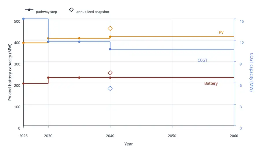
The first case is a greenfield annualized 2040 snapshot: it sees only target-year conditions and annualizes capital costs into one year. The second case is a linked pathway from 2026 to 2040 with a model horizon to 2060. The pathway starts with 15 MW of inherited CCGT capacity installed in 2025, so it can use a sunk gas unit during the transition but must also respect retirement and replacement logic.
Data Sources
The technology-cost values below are illustrative values derived from Danish Energy Agency technology-data catalogues:
- PV and CCGT values are based on Technology Data for Generation of Electricity and District Heating.
- Battery values are based on Technology Data for Energy Storage.
Fuel costs, direct emission factors, the emissions cap, and the synthetic PV profile are scenario assumptions chosen to keep the example compact.
Model
The model uses a full-year hourly mesh with 8760 timesteps. Dispatch-dependent quantities such as fuel use, cycling costs, and direct emissions are therefore already annual totals. Fixed costs stay annual.
using EnergyPathway
using DataFrames: DataFrame
using HiGHS
using JuMP: @constraint, set_silent

# Assumptions are kept together in a dictionary. For an example, this is easier
# to scan and modify than a long sequence of unrelated top-level constants.
assumptions = Dict(
    # These are the pathway decision years. Capacity can change in these years,
    # while intermediate years inherit the previous decision year's capacity.
    :snapshot_years => [2026, 2030, 2035, 2040],
    # The economic horizon extends beyond the last decision year so investments
    # made in 2040 still carry value and costs over their useful project life.
    :end_year => 2060,
    :discount_rate => 0.05,
    :load_mw => 70.0,
    :hours_per_year => 8760,
    :emission_cap_t => Dict(:start => 30_000.0, :target => 15_000.0),
    # Initial capacity is represented as (installation year, component name,
    # capacity, lifetime). Here the inherited CCGT is alive in 2026.
    :existing_capacity => [(2025, "CCGT", 15.0, 15)],
    :technology => Dict(
        # Capex and fixed O&M are illustrative 2040-style values based on the
        # Danish Energy Agency technology-data catalogues. Fuel costs and direct
        # emission factors are scenario assumptions for this example.
        "PV" => Dict(:capex => 320_000.0, :fom => 8_100.0, :lifetime => 40),
        "battery" => Dict(
            :capex => 771_200.0,
            :fom => 8_675.898,
            :lifetime => 30,
            :duration_h => 4.0,
            :cycling_cost => 1.0,
            :efficiency_in => 0.92,
            :efficiency_out => 0.92,
        ),
        "CCGT" => Dict(
            :capex => 866_648.765,
            :fom => 28_604.726,
            :lifetime => 25,
            :variable_cost => 55.207,
            :co2_t_per_mwh => 0.360,
        ),
    ),
)

first_year(case=assumptions) = first(case[:snapshot_years])
target_year(case=assumptions) = last(case[:snapshot_years])

# Linear interpolation is used for the policy trajectory, not for capacities.
# Pathway capacities are carried forward between explicit decision years.
function lerp(year, start_year, end_year, start_value, end_value)
    share = (year - start_year) / (end_year - start_year)
    return start_value + share * (end_value - start_value)
end

function emission_cap(year, case=assumptions)
    # The cap tightens from 2026 to 2040, then stays fixed through the economic
    # horizon. This keeps post-2040 renewals subject to the target constraint.
    if year <= target_year(case)
        return lerp(
            year,
            first_year(case),
            target_year(case),
            case[:emission_cap_t][:start],
            case[:emission_cap_t][:target],
        )
    else
        return case[:emission_cap_t][:target]
    end
end

function annuity(capex, lifetime, case=assumptions)
    # The annualized snapshot cannot decide when construction happens, so capex
    # is converted to a recurring fixed charge using the same discount rate.
    rate = case[:discount_rate]
    return capex * rate / (1.0 - (1.0 + rate)^(-lifetime))
end

function yearly_mesh(case=assumptions)
    # A default TimeMesh represents the full model year at hourly resolution.
    return TimeMesh()
end

function load_profile(case=assumptions)
    # A flat load keeps the comparison focused on capacity-expansion logic.
    return fill(case[:load_mw], case[:hours_per_year])
end

function pv_profile(case=assumptions)
    # This synthetic profile gives PV both daily and seasonal structure without
    # pulling an external weather file into the documentation example.
    hours = 0:(case[:hours_per_year] - 1)
    values = [
        0.88 *
        max(0.0, sin(pi * ((hour % 24) - 6) / 12)) *
        (0.78 + 0.22 * sin(2pi * (div(hour, 24) - 80) / 365))
        for hour in hours
    ]
    return [value < 1e-8 ? 0.0 : value for value in values]
end

function pathway_asset_behaviors(port_name, tech_data)
    # Pathway assets have explicit deployment, retirement, lifetime, and
    # one-time capex behavior, so costs are paid when capacity is built.
    return [
        VariableCapacity(port_name, energy),
        VariableDeployment(port_name, energy),
        VariableRetirement(port_name, energy),
        Lifetime(tech_data[:lifetime]),
        SingleCost(
            :capex,
            :deployment,
            port_name,
            energy,
            tech_data[:capex],
            # Split capex across the year before commissioning and the
            # commissioning year to mimic a simple construction-payment profile.
            Dict(-1 => 0.30, 0 => 0.70),
        ),
        FixedCost(:fom, port_name, energy, tech_data[:fom]),
    ]
end

function annualized_asset_behaviors(port_name, tech_data, case=assumptions)
    # The snapshot comparison has no deployment history, so each MW of capacity
    # carries an annualized investment charge instead of one-time capex.
    return [
        VariableCapacity(port_name, energy),
        FixedCost(
            :annualized_capex,
            port_name,
            energy,
            annuity(tech_data[:capex], tech_data[:lifetime], case),
        ),
        FixedCost(:fom, port_name, energy, tech_data[:fom]),
    ]
end

function asset_behaviors(mode, port_name, tech_data, case=assumptions)
    # Both cases use the same physical technologies; only the investment
    # accounting changes between snapshot and pathway formalisms.
    if mode == :pathway
        return pathway_asset_behaviors(port_name, tech_data)
    elseif mode == :annualized
        return annualized_asset_behaviors(port_name, tech_data, case)
    else
        throw(ArgumentError("unknown investment mode: $mode"))
    end
end

function add_facility_system!(snapshot, year; mode, case=assumptions)
    tech = case[:technology]
    carrier = EnergyCarrier("electricity", sim(snapshot))
    # Curtailment on the plant bus lets PV overproduction be spilled instead of
    # forcing infeasible generation during high-solar, low-storage hours.
    bus = Node("plant_bus", carrier; rule=:curtailed)

    # The facility is represented as a fixed electrical baseload.
    # The site is islanded: there is deliberately no grid-purchase component.
    load = Component("facility_load", Demand(carrier, load_profile(case)))
    connect!(snapshot, load, bus)

    # PV output is limited by the normalized production profile and its chosen
    # capacity on the output port.
    pv = Component(
        "PV",
        ProfileSource(carrier, pv_profile(case)),
        asset_behaviors(mode, "output", tech["PV"], case),
    )
    connect!(snapshot, pv, bus)

    # The storage capacity variable is on the input port. Duration links charge
    # power to energy capacity and output capability inside Nosy.
    battery = Component(
        "battery",
        BasicStorage(
            carrier;
            eff_i=tech["battery"][:efficiency_in],
            eff_o=tech["battery"][:efficiency_out],
            simplified=true,
        ),
        vcat(
            asset_behaviors(mode, "input", tech["battery"], case),
            [
                Duration(tech["battery"][:duration_h]),
                VariableCost(:cycling, "output", energy, tech["battery"][:cycling_cost]),
            ],
        ),
    )
    connect!(snapshot, battery, bus)

    # CCGT is the dispatchable backstop. Its investment treatment still depends
    # on the selected mode, just like PV and battery.
    ccgt = Component(
        "CCGT",
        DispatchableSource(carrier),
        vcat(
            asset_behaviors(mode, "output", tech["CCGT"], case),
            [
                VariableCost(
                    :fuel,
                    "output",
                    energy,
                    tech["CCGT"][:variable_cost],
                ),
            ],
        ),
    )
    connect!(snapshot, ccgt, bus)

    # Because the mesh is hourly for a full year, aggregating CCGT output gives
    # annual MWh, which can be multiplied directly by the emission factor.
    annual_emission =
        tech["CCGT"][:co2_t_per_mwh] *
        balance(snapshot, "CCGT", :output, energy; collapse=true, aggregate=true)

    @constraint(model(sim(snapshot)), annual_emission <= emission_cap(year, case))

    return snapshot
end

function build_annualized_snapshot(case=assumptions)
    # The comparison snapshot only models the target year. Discounting is set to
    # zero because all investment costs have already been annualized.
    opt = PathOpt(
        [target_year(case)];
        discountrate=0.0,
        baseyear=target_year(case),
        endyear=target_year(case),
        mesh=yearly_mesh(case),
    )
    snapshot = Path(HiGHS.Optimizer, opt)
    set_silent(model(snapshot))

    add_facility_system!(
        snapshot[target_year(case)],
        target_year(case);
        mode=:annualized,
        case=case,
    )
    optimize!(snapshot, cost(snapshot))

    return extract(snapshot)
end

function build_pathway(case=assumptions)
    # The pathway shares one JuMP model across all decision-year snapshots and
    # receives inherited capacity through the initial-capacity data.
    opt = PathOpt(
        case[:snapshot_years];
        discountrate=case[:discount_rate],
        baseyear=first_year(case),
        endyear=case[:end_year],
        mesh=yearly_mesh(case),
        ini=case[:existing_capacity],
    )
    pathway = Path(HiGHS.Optimizer, opt)
    set_silent(model(pathway))

    # Each decision year has the same physical system, with year-specific policy
    # constraints and pathway behaviors linking capacities through time.
    for year in case[:snapshot_years]
        add_facility_system!(pathway[year], year; mode=:pathway, case=case)
    end

    optimize!(pathway, cost(pathway))

    return extract(pathway)
end

function solve_facility_transition(case=assumptions)
    return build_annualized_snapshot(case), build_pathway(case)
end

function annual_flow_mwh(snapshot, component_name, case=assumptions)
    return balance(snapshot, component_name, :output, energy; collapse=true, aggregate=true)
end

function annual_emission_t(snapshot, case=assumptions)
    tech = case[:technology]
    return tech["CCGT"][:co2_t_per_mwh] * annual_flow_mwh(snapshot, "CCGT", case)
end

clean_mw(value) = abs(value) < 1e-6 ? 0.0 : value
rounded_mw(value) = round(clean_mw(value); digits=3)

function capacity_summary(snapshot, pathway, case=assumptions)
    rows = NamedTuple[]

    # Put the one-year snapshot next to each pathway decision year so the final
    # 2040 end state can be compared with the dynamic transition.
    push!(rows, (
        case="annualized snapshot",
        year=target_year(case),
        PV_MW=rounded_mw(capacity(snapshot, "PV", target_year(case))),
        battery_MW=rounded_mw(capacity(snapshot, "battery", target_year(case))),
        CCGT_MW=rounded_mw(capacity(snapshot, "CCGT", target_year(case))),
    ))

    for year in case[:snapshot_years]
        push!(rows, (
            case="pathway $(case[:end_year])",
            year=year,
            PV_MW=rounded_mw(capacity(pathway, "PV", year)),
            battery_MW=rounded_mw(capacity(pathway, "battery", year)),
            CCGT_MW=rounded_mw(capacity(pathway, "CCGT", year)),
        ))
    end

    return DataFrame(rows)
end

function emission_summary(snapshot, pathway, case=assumptions)
    # Emissions are reported against the cap to show which periods bind and how
    # the inherited gas capacity is constrained over time.
    rows = NamedTuple[(
        case="annualized snapshot",
        year=target_year(case),
        emission_t=round(annual_emission_t(snapshot[target_year(case)], case); digits=1),
        cap_t=emission_cap(target_year(case), case),
    )]

    for year in case[:snapshot_years]
        push!(rows, (
            case="pathway $(case[:end_year])",
            year=year,
            emission_t=round(annual_emission_t(pathway[year], case); digits=1),
            cap_t=emission_cap(year, case),
        ))
    end

    return DataFrame(rows)
end

snapshot, pathway = solve_facility_transition();
nothing

# output
Capacity Summary
julia> capacity_summary(snapshot, pathway)
5×5 DataFrame
 Row │ case                 year   PV_MW    battery_MW  CCGT_MW
     │ String               Int64  Float64  Float64     Float64
─────┼──────────────────────────────────────────────────────────
   1 │ annualized snapshot   2040  455.148     247.283    5.223
   2 │ pathway 2060          2026  387.768     197.447   15.0
   3 │ pathway 2060          2030  408.863     225.067   11.782
   4 │ pathway 2060          2035  408.863     225.067   11.782
   5 │ pathway 2060          2040  416.495     225.067   10.737
The annualized snapshot builds directly for 2040. The pathway builds less PV and uses more CCGT early on because the inherited 15 MW unit is already present and does not carry new investment cost.
Emission Summary
julia> emission_summary(snapshot, pathway)
5×4 DataFrame
 Row │ case                 year   emission_t  cap_t
     │ String               Int64  Float64     Float64
─────┼─────────────────────────────────────────────────
   1 │ annualized snapshot   2040      2508.1  15000.0
   2 │ pathway 2060          2026     28597.4  30000.0
   3 │ pathway 2060          2030     15948.0  25714.3
   4 │ pathway 2060          2035     15948.0  20357.1
   5 │ pathway 2060          2040     15000.0  15000.0
The emissions table is useful for checking that the inherited gas unit is not a free pass: even when its investment cost is sunk, its dispatch is still limited by the direct-emissions cap in each modeled year.